This post is part of a series on Mohammad Anwar’s excellent Weekly Challenge, where hackers submit solutions in Perl, Raku, or any other language, to two different challenges every week. (It’s a lot of fun, if you’re into that sort of thing.)
For the first task this week, you’re given a list of numbers and simply have to return the number that is closest to zero. Core module List::Util helps us here.
sub zero_friend { min map abs, @_ }
There isn’t much explanation to be offered, here. We first map our list of arguments (@_) to their absolute values, and then return the minimum of that.
This post is part of a series on Mohammad Anwar’s excellent Weekly Challenge, where hackers submit solutions in Perl, Raku, or any other language, to two different challenges every week. (It’s a lot of fun, if you’re into that sort of thing.)
Task 1: Balanced Strings
Our first task this week is to take a string matching /^[a-z0-9]$/ and produce the lexicographically smallest string with alternating letters and numbers. If it’s not possible to produce a string without two letters or numbers in a row, return ''.
For example, 1bca2 should return a1b2c, whereas 1a23 returns the empty string because there are too many numbers vs. letters.
Easy enough. For this I’ll use mesh() from the core module List::Util. mesh() takes two (or more) arrays and gives you alternating values from each of them. Perfect for what we need. We just need to make sure we have the same number of letters and numbers (or one more).
use List::Util qw< mesh >;
no warnings 'uninitialized';

sub balanced {
    die "`$_[0]' must contain [a-z0-9]" if $_[0] !~ /^[a-z0-9]*$/;
    my ($one, $two) = ([], []);

    push @{ /\d/ ? $one : $two }, $_ for sort split '', $_[0];
    return "" if abs(@$one - @$two) > 1; # Unbalanced

    join '', mesh sort { @$b <=> @$a } $one, $two;
}
That last sort { @$b <=> @$a } $one, $two is not sorting the elements of $one and $two! It’s sorting the order of the arrays themselves, putting the one with more elements first. This ensures we don’t have to have two numbers or letters in a row. For example, if we have abc and 1234, we had better start with a number, or we’d end up with a1b2c34, which is invalid.
Task 2: Max Score
This task is a partitioning problem. Given a string of 1s and 0s, we’re to split it into two non-empty substrings. The score is the sum of 0s in the left string, plus 1s in the right string.
This post is part of a series on Mohammad Anwar’s excellent Weekly Challenge, where hackers submit solutions in Perl, Raku, or any other language, to two different challenges every week. (It’s a lot of fun, if you’re into that sort of thing.)
I’ve recently moved all the sites I host to a new server, including ry.ca, and realized it’s been far too long since I wrote a blog post. And, indeed, far too long since I’ve had time for any sort of recreational programming. So let’s fix that!
Task 1: My Keyboard is Broken
This task posits that age old question: which words could I still type if my keyboard was broken? For example, if the o key on your keyboard is broken, you can (correctly) type help, but not keyboard or broken.
The solution (made possible to code without an o for your convenience):
sub pssible($str, @brken) {
    grep !/[@brken\0]/i, split /\s+/, $str
}
This post is part of a series on Mohammad Anwar’s excellent Weekly Challenge, where hackers submit solutions in Perl, Raku, or any other language, to two different challenges every week. (It’s a lot of fun, if you’re into that sort of thing.)
Task 1 › Large Numbers
The first task this week has us taking a list of numbers and finding the permutation whose concatenation gives the largest number. For example: largest(20,3) = 320.
At first, I thought I might get away with a greedy join('', reverse sort @ints) but the greedy approach doesn’t work in this case. For example, join('', reverse sort(5, 50, 51)) would give 51505, but the correct answer is 55150. So, a more deliberate approach is needed. However, see the update below this section!
This post is part of a series on Mohammad Anwar’s excellent Weekly Challenge, where hackers submit solutions in Perl, Raku, or any other language, to two different challenges every week. (It’s a lot of fun, if you’re into that sort of thing.)
(Yes, the title is a reference to the 2006 Zach Snyder film.)
I’d say I can hardly believe we’ve hit the 300th week in a row of the Weekly Challenge. But, then again, knowing a little bit about the persistence and work ethic of Mohammad Anwar, it’s really no surprise. Let’s keep this going for a good while longer!
Task 1: Beautiful Arrangements
The first task this week has us take a positive $integer and look at every permutation @P of the numbers 1..$int. We then return the count of permutations where every element in @P is either divisible by its 1-based index, or the index is divisible by the element.
This post is part of a series on Mohammad Anwar’s excellent Weekly Challenge, where hackers submit solutions in Perl, Raku, or any other language, to two different challenges every week. (It’s a lot of fun, if you’re into that sort of thing.)
OK, the title might need some explaining: Both tasks this week have us looking through lists of numbers and doubling some of them.
Task 1 › Double Exist
Task 1’s premise is simple enough: we take in a list of @ints and return a true value if the list contains a number and its double.
We also have the restriction that the same list element cannot be its own double. Zero is the only integer this can happen with. For example, (0) returns false even though 2×0 = 0, but (0,0) returns true because the second zero is a different list element.
We can solve this in O(n) time with a little bit of housekeeping: we will track whether we have seen the double of a number, and the half of a number (if that number is even). Tracking both doubles and halves ensures that we will find the 2k whether it comes before or after k in the list.
This post is part of a series on Mohammad Anwar’s excellent Weekly Challenge, where hackers submit solutions in Perl, Raku, or any other language, to two different challenges every week. (It’s a lot of fun, if you’re into that sort of thing.)
Task 1 – 3rd Maximum
Task 1 this week is to take a list of integers and find the 3rd unique maximum value, or if there are fewer than 3 unique values, return the overall maximum. Examples:
Integers
3rd Maximum
5, 6, 4, 1
4
4, 5
5
1, 2, 2, 3
1
To accomplish this, I just sort the input integers and get the uniq list from that (from core module List::Util). The sort is O(n log n), but it’s only done once, so that’s our overall complexity.
It would also be possible to use a sliding window for this, but then every insert would be more expensive, up to O(wn) complexity where w is the window size. For constant w where w << n, this might be a win, but Perl’s slow looping speed might make that constant factor dominate, and the code would have been more complex. Still, it could have been fun to experiment with some profiling, given more time.
The general case solution is extremely simple:
sub nth_max {
    my $n = shift;
    my @uniq_sorted = uniq sort { $b <=> $a } @_;

    $uniq_sorted[ @uniq_sorted >= $n ? $n - 1 : 0 ]
}
This post is part of a series on Mohammad Anwar’s excellent Weekly Challenge, where hackers submit solutions in Perl, Raku, or any other language, to two different challenges every week. (It’s a lot of fun, if you’re into that sort of thing.)
The first challenge this week has us finding the count of words that appears exactly once in each of two lists. For example:
('Perl', 'is', 'my', 'friend'), ('Perl', 'and', 'Raku', 'are', 'friend') Should return 2 since Perl and friend appear once in each list. But,
('twice', 'twice'), ('twice') should return 0, since twice appears more than once in one of the arrays.
Since it was easy, I opted to support an arbitrary number of arrays instead of just two. It would of course be trivial to limit the input to two arrays. I also support scalar and list context, so you can easily get just the count (as the task asks), or call the function in list context to get the actual list of common words.
Since my algorithm is O(n), I do not return sorted results by default, as a minor optimization. If stable output is needed, simply sort the result.
This post is part of a series on Mohammad Anwar’s excellent Weekly Challenge, where hackers submit solutions in Perl, Raku, or any other language, to two different challenges every week. (It’s a lot of fun, if you’re into that sort of thing.)
I thought I’d take the rare (for me) step of implementing this week’s challenges in Python as well as Perl.
Happy Canada Day!
Task 1 – Complete Day
The first task has us look through a list of hours and count the number of pairs that add up to a multiple of 24.
Perl
My first version was done in a compact functional style, which may be more challenging for Perl novices:
Reading from bottom up as usual, we iterate through the indices of @_ (our hours array) and map { ... } each index to a list of array refs from index to end of list. So, given (1, 2, 3, 4, 5), we would expect to get the following list for this intermediate step:
The first map { ... } then splits this into $m, with the rest of the values in @$_ (note the shift). $m and @$_ are effectively car and cdr if you recall your lisp (although not many of us still do, I suppose).
There is an inner map { ... } that then adds $m to every value in @$_, and maps to 1 if it is a multiple of 24 and 0 if it is not. sum0 from the core module List::Util simply adds them all up to get a count.
More readable example
A more readable version is as follows:
sub complete_day {
    my $count = 0;
    while (my $m = shift) {
        $count += sum0 map { ($m + $_) % 24 == 0 } @_
    }

    $count
}
This one simply maintains a $count as it goes, peeling off a new $m each time through the while() { ... } loop, with a similar inner map { ... } as before.
For Perl Weekly Challenge code, I like to show off some different programming styles. Which one I would actually use in production is another question entirely.
Python
I didn’t think too hard about this one:
def complete_day(hours):
    count = 0
    for i, m in enumerate(hours):
        for n in filter(lambda n: ((m + n) % 24 == 0), hours[i+1:]):
            count += 1

    return(count)
This works similarly to the second Perl example.
Task 2 – Maximum Frequency
The second task this week has us looking at a list of values, finding the maximum frequency of any particular value, and then returning the total number of items with that maximum frequency. This is best demonstrated by example.
Given (1, 2, 2, 4, 1, 5), both 1 and 2 occur twice, so the maximum frequency is 2. Since there are two different values with that frequency, we would return 2 x 2 = 4.
Given (1, 2, 2, 4, 6, 1, 5, 6), 1, 2, and 6 occur twice, so the maximum frequency is 2, but now there are three different values with that frequency, so we return 3 x 2 = 6.
Perl
sub max_freq {
    my %freq; # Frequency table
    $freq{$_}++ for @_;

    my $max_freq = max values %freq; # Maximal frequency

    $max_freq * grep { $_ == $max_freq } values %freq;
}
There are three essential steps here. First, we build a %frequency table, mapping values to the number of times they appear. Then we find the $max_freq with a quick pass through the values of that hash.
The final answer is generated by multiplying $max_freq by the count of values where the frequency is equal to $max_freq. Easy!
Python
def max_freq(ints):
    # Annoying special case for empty list
    if len(ints) == 0:
        return(0)

    # Build the frequency table (freq[n] = # of times n is in ints)
    freq = {}
    for n in ints: freq[n] = freq.setdefault(n,0) + 1

    max_freq = max(freq.values()) # Maximal frequency

    return(sum(filter(lambda x: x == max_freq, freq.values())))
This roughly follows the Perl code, although we need a special case for empty lists (otherwise we get an error).
This post is part of a series on Mohammad Anwar’s excellent Weekly Challenge, where hackers submit solutions in Perl, Raku, or any other language, to two different challenges every week. (It’s a lot of fun, if you’re into that sort of thing.)
This week’s tasks have a little bit more meat on their bones, which I quite enjoyed. They are user-submitted, as well, and it’s always fun to see what people come up with when submitting tasks.
Task 1 – Banking Day Offset
This task comes from the mind of Lee Johnson. Here, we’re given the following inputs:
Number of days [$offset]
Start date [$start_date]
List of dates which are holidays (optional) [@holidays]
From that, we’re supposed to return the date that is $offset working days from the $start_date, ignoring weekends and @holidays. This is straightforward. I opted to use the core Perl module Time::Piece to get the day of the week. There are about n + 1 different ways to do that, though.
The function starts with some initialization:
sub bank_holiday_ofs {
    my ($start_date, $offset, @holidays) = @_;

    my $t = Time::Piece->strptime($start_date => $date_fmt) - 86400;

    my %holiday = map { $_ => 1 } @holidays;
    $offset++; # Account for today
The %holiday hash simply maps the dates to a true value so $holiday{$date} will be true iff$date is in @holidays. The $offset variable gets an extra kick to account for the current day.
From here, we loop until $offset is zero:
    while ($offset) {
        $t += 86400; # Advance day
        $offset-- unless $t->wday == 1 or $t->wday == 7
                      or $holiday{ $t->strftime($date_fmt) };
    }
From years of frequent use, 86,400 has sufficient semantic meaning as “1 day” that I’m not bothered about the naughty magic number. If that’s not your style, Time::Seconds has a ONE_DAY constant.
The loop is simple. Add a day, and then subtract a day from $offset unless it’s a weekend or holiday.
We are also required to handle escaped quotes (\") and (optionally) multiline tags. I wrote a pure-Perl parser that handles all of this. It’s easiest to think of in two parts:
Top level line parser
This is the part that takes in a line of text and decides what to do with it. First, let’s define our $Open and $Close tags:
my ($O, $C) = (qr/^\s*\{\%\s*/, qr/\s*\%\}\s*$/); # Tokens gobble whitespace
I could have just done a simple {% and %} set, but I wanted to allow optional whitespace. A recurring theme you’ll see with my solution (and my parsers in general) is that I tend to be permissive with inputs, but precise with outputs.
Now I loop through each line of input (in this case, the __DATA__ block):
  for (<DATA>) {
      chomp;

      if ($id) {
          if (/${O}end$id${C}/) {
              $id{$id}{text} = @text > 1 ? [ @text ] : $text[0];
              @text = ();
              $id = undef;
          } else {
              push @text, $_
          }
      }
      elsif (/${O}(?<id>\w+)\s+(?<fields>.+?)${C}/) {
          die "No end token found for <$id>" if $id and @text;
          $id = $+{id};
          die "Duplicate id <$id>" if exists $id{$id};
          $id{$id} = { name => $id, fields => parse_fields($+{fields}) };
      }
      else {
          die "Invalid line: <$_>";
      }
  }
The way this loop works is, if $id is defined, we’ve already seen an open {% tag and we’re expecting either a line of text, or the {% endid %} closing tag, so we look for those and handle them accordingly.
Otherwise, we expect to see a single line {% id key=value, ... %} record or the start of a multi-line record, so we look for that. We pass the key/value portion of the record to the parse_fields() sub, which we’ll look at next.
parse_fields(): The key/value (kv) parser
It might seem like parsing keys and values would be the easy part, and if not for Gabor’s requirement to handle escaped quotes, it might have been. There are several ways I could have tackled this, from tricky eval()s to full-blown grammars, but for my purposes here (and because I felt like it), I decided to implement a simple state machine.
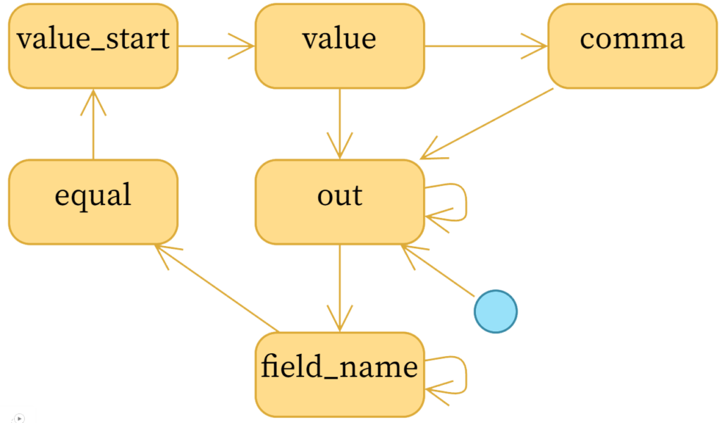
Finite state machines can be described by a directed graph whose vertices contain the possible states the system can be in, and edges are the possible state transitions. To parse the kv pairs as described by this task, the following state machine will do the trick:
State diagram for parsing key/value pairs.
Note: To avoid a cluttered diagram, I’ve omitted arrows on most states that point to themselves, except for field_name and out. It so happens that every state in this particular system can have itself as the next state.
We effectively start from the out state, meaning we are outside of a key/value pair and are waiting for the start of the next key name. Once we see a word character (\w), we go to the field_name state and stay there until we’ve gobbled up all of the \w characters, and then we look for an equal sign. We similarly trundle through the states to find the start of the value (value_start), the value itself, then a comma, and back to out for the next field. We can stop at any time.
One way to implement simple state machines is by simply having a $state variable that you set to the name of the state you’re in, and an if ... elsif ... chain to handle the state transitions. For more complicated, or dynamic state machines, you might reach for one of the many CPAN modules for finite state machines (FSM). But I wanted to show you how it can be done without any help.
My parse_fields() function iterates over the input string character by character. First, we have some top level variables to keep track of:
      my %fields;
      my $state = 'out'; # Outside of KV pair
      my $backslash = 0; # Substate for whether we're backslashed
      my $name = undef;  # Field name
      my $value = undef; # Field value
      my $expected_closing_quote; # If defined, value must end with this
Our output will be %fields. The $backslash variable actually captures a parallel state of whether the last character was a backslash (1), whether the current character was escaped (2), or whether neither of those things is true (0). I might have used named values instead, but this made sufficient sense to me.
I decided values could be optionally quoted, by single ('), double (") or nothing, but that the closing quote had to match the opening quote. So that’s what $expected_closing_quote keeps track of.
I do use eval here, but you’ll note it’s done in a safe manner, as I only ever pass two characters to eval, and the first character is a backslash. I could have built up my own hash of slash characters, but that would be error prone and require updating with the language.
If the current character is a backslash, we just set $backslash and go to the next character. If the previous character was a backslash, we do the eval to get the unescaped character. We then set $backslash to 2, which is used when we’re looking for quotes, to avoid ending the value on an escaped quote.
Here’s what a typical state handler looks like:
          # Handle the value, with optional quotes and escape sequences
          elsif ($state eq 'value_start') {
              next if /\s/;
              if (/['"]/ and not $backslash) {
                  $expected_closing_quote = $_;
                  $state = 'value';
                  $value = '';
                  next;
              }
              $value = $_;
              $state = 'value';
          }
That is the value state. You’ll see that has the logic I just talked about; if we see our $expected_closing_quote and it wasn’t $backslashed, or we see whitespace and the value is not quoted at all, we have reached the end of the value. So we set $fields{$name} = $value (that’s now part of our return value), set our next state to comma, and go to the next character.
On the other hand, if none of those conditions were true, that means we’re still inside the value, so we append the character to $value and continue. (The value state points to itself.)
I won’t show all of the states here, as the above should give you the flavor of it, but of course you can see my full solution here.
All in all, it’s decently robust for a PWC task solution, but a production version could certainly use some better error checking and reporting. Invalid inputs are mostly handled fairly gracefully, but the resulting output might be confusing.